Download the notebook here! Interactive online version:

import sys
import respy as rp
import numpy as np
sys.path.insert(0, "python")
from auxiliary import plot_observed_choices  # noqa: E402
from auxiliary import plot_time_preference  # noqa: E402
from auxiliary import plot_policy_forecast  # noqa: E402

Structural microeconometrics

Computational modeling in economics

• provide learning opportunities

• assess importance of competing mechanisms

• predict the effects of public policies

Eckstein-Keane-Wolpin (EKW) models}

• understanding individual decisions

  • human capital investment

  • savings and retirement

• predicting effects of policies

  • welfare programs

  • tax schedules

Components

• economic model

• mathematical formulation

• calibration procedure

Economic model

Decision problem

\[\begin{split}\begin{array}{ll} t = 1, .., T& \text{decision period} \\ s_t\in S & \text{state} \\ a_t\in A & \text{action} \\ a_t(s_t) & \text{decision rule} \\ r_t(s_t, a_t) & \text{immediate reward}\\ \end{array}\end{split}\]

\[\begin{split}\begin{array}{ll} \pi = (a^\pi_1(s_1), .., a^\pi_T(s_T)) & \text{policy}\\ \delta & \text{discount factor} \\ p_t(s_t, a_t) & \text{conditional distribution} \end{array}\end{split}\]

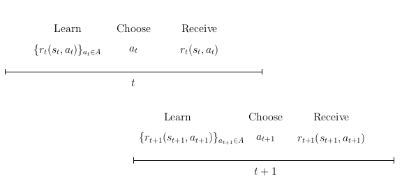
Individual’s objective

\[\max_{\pi \in\Pi} E_{s_1}^\pi\left[\left.\sum^{T}_{t = 1} \delta^{t - 1} r_t(s_t, a^\pi_t(s_t))\,\right\vert\,\mathcal{I}_1\,\right]\]

Mathematical formulation

Policy evaluation

\[\begin{split}v^\pi_t(s_t) \equiv E_{s_t}^\pi\left[\left.\sum^{T - t}_{j = 0} \delta^j\, r_{t + j}(s_{t + j}, a^\pi_{t + j}(s_{t + j})) \,\right\vert\,\mathcal{I}_t\,\right]\\\end{split}\]

Inductive scheme

\[v^\pi_t(s_t) = r_t(s_t, a^\pi_t(s_t)) + \delta\,E^\pi_{s_t} \left[\left.v^\pi_{t + 1}(s_{t + 1}) \,\right\vert\,\mathcal{I}_t\,\right]\]

Optimality equations

\[v^{\pi^*}_t(s_t) = \max_{a_t \in A}\bigg\{ r_t(s_t, a_t) + \delta\, E^{\pi^*}_{s_t} \left[\left.v^{\pi^*}_{t + 1}(s_{t + 1})\,\right\vert\,\mathcal{I}_t\,\right] \bigg\}\]

Calibration procedure

Data

\[ \begin{align}\begin{aligned}\begin{split} \mathcal{D} = \{a_{it}, x_{it}, r_{it}: i = 1, ... , N; t = 1, ... , T_i\}\\\end{split}\\**State variables}**\end{aligned}\end{align} \]

• \(s_t = (x_t, \epsilon_t)\)

  • \(x_t\) observed

  • \(\epsilon_t\) unobserved

Procedures

• likelihood-based

  \[\hat{\theta} \equiv argmax_{\theta \in \Theta} \prod^N_{i= 1} \prod^{T_i}_{t= 1}\, p_{it}(a_{it}, r_{it} \mid x_{it}, \theta)\]

• simulation-based

  \[\hat{\theta} \equiv argmin_{\theta \in \Theta} (M_D - M_S(\theta))' W (M_D - M_S(\theta))\]

Example

Seminal paper

• Keane, M. P., & Wolpin, K. I. (1994). The solution and estimation of discrete choice dynamic programming models by simulation and interpolation: Monte Carlo evidence. Review of Economics and Statistics, 76 (4), 648–672.

Model of occupational choice

• 1,000 individuals starting at age 16

• life cycle histories

  • school attendance

  • occupation-specific work status

• wages

Labor market

\[\begin{split}r_t(s_t, 1) = w_{1t} = \exp\{ \underbrace{\alpha_{10}}_{\text{endowment}} + \underbrace{\alpha_{11} g_t}_{\text{schooling}} + \underbrace{\alpha_{12}e_{1t} + \alpha_{13}e^2_{1t}}_{\text{own experience}} \\ + \underbrace{\alpha_{14}e_{2t} + \alpha_{15}e^2_{2t}}_{\text{other experience}} + \underbrace{\epsilon_{1t}}_{\text{shock}}\}\end{split}\]

The same setup applies to the second occupation.

Schooling

\[\begin{split}r_t(s_t, 3) = \underbrace{\beta_0}_{\text{taste}} - \underbrace{\beta_1 I[\,g_t \geq 12\,]}_{\text{direct cost}} - \underbrace{\beta_2 I[\,a_{t - 1} \neq 3\,]}_{\text{reenrollment effort}} + \underbrace{\epsilon_{3t}}_{\text{shock}} \\\end{split}\]

Home

\[r_t(s_t, 4) = \underbrace{\gamma_0}_{\text{taste}} + \underbrace{\epsilon_{4t}}_{\text{shock}}\]

State space

\[s_t = \{g_t,e_{1t},e_{2t},a_{t - 1},\epsilon_{1t},\epsilon_{2t},\epsilon_{3t},\epsilon_{4t}\}\]

Transitions

• observed state variables

  \[\begin{split}e_{1,t+1} = e_{1t} + I[\,a_t = 1\,] \\ e_{2,t+1} = e_{2t} + I[\,a_t = 2\,] \\ g_{t+1} = g_{t\phantom{2}} + I[\,a_t = 3\,]\end{split}\]

• unobserved state variables

  \[\{\epsilon_{1t},\epsilon_{2t},\epsilon_{3t},\epsilon_{4t}\} \sim N(0, \Sigma)\]

params, options = rp.get_example_model("kw_94_two", with_data=False)

How is the economy parametrized?

params.head()

		value	comment
category	name
delta	delta	0.9500	discount factor
wage_a	constant	9.2100	log of rental price
	exp_edu	0.0400	return to an additional year of schooling
	exp_a	0.0330	return to same sector experience
	exp_a_square	-0.0005	return to same sector, quadratic experience

How are the options set?

options

{'estimation_draws': 200,
 'estimation_seed': 500,
 'estimation_tau': 500,
 'interpolation_points': -1,
 'n_periods': 40,
 'simulation_agents': 1000,
 'simulation_seed': 132,
 'solution_draws': 500,
 'solution_seed': 1,
 'monte_carlo_sequence': 'random',
 'core_state_space_filters': ["period > 0 and exp_{choices_w_exp} == period and lagged_choice_1 != '{choices_w_exp}'",
  "period > 0 and exp_a + exp_b + exp_edu == period and lagged_choice_1 == '{choices_wo_exp}'",
  "period > 0 and lagged_choice_1 == 'edu' and exp_edu == 0",
  "lagged_choice_1 == '{choices_w_wage}' and exp_{choices_w_wage} == 0",
  "period == 0 and lagged_choice_1 == '{choices_w_wage}'"],
 'covariates': {'constant': '1',
  'exp_a_square': 'exp_a ** 2',
  'exp_b_square': 'exp_b ** 2',
  'at_least_twelve_exp_edu': 'exp_edu >= 12',
  'not_edu_last_period': "lagged_choice_1 != 'edu'"}}

We can now simulate a dataset and look at the individual decisions.

simulate_func = rp.get_simulate_func(params, options)
plot_observed_choices(simulate_func(params))

Mechanisms

def time_preference_wrapper_kw_94(simulate_func, params, value):
    policy_params = params.copy()
    policy_params.loc[("delta", "delta"), "value"] = value
    policy_df = simulate_func(policy_params)

    edu = policy_df.groupby("Identifier")["Experience_Edu"].max().mean()

    return edu

Now we can iterate over a grid of discount factors.

deltas = np.linspace(0.945, 0.955, 10)
edu_level = list()

for i, delta in enumerate(deltas):
    stat = time_preference_wrapper_kw_94(simulate_func, params, delta)
    edu_level.append(stat)

plot_time_preference(deltas, edu_level)

Policy forecast

def tuition_policy_wrapper_kw_94(simulate_func, params, tuition_subsidy):
    policy_params = params.copy()
    policy_params.loc[("nonpec_edu", "at_least_twelve_exp_edu"), "value"] += tuition_subsidy
    policy_df = simulate_func(policy_params)

    edu = policy_df.groupby("Identifier")["Experience_Edu"].max().mean()

    return edu

Now we can iterate over a grid of tuition subsidies.

subsidies = np.linspace(0, 1500, num=10, dtype=int, endpoint=True)
edu_level = list()

for i, subsidy in enumerate(subsidies):
    stat = tuition_policy_wrapper_kw_94(simulate_func, params, subsidy)
    edu_level.append(stat)

plot_policy_forecast(subsidies, edu_level)